EEGPlot.jl

A julia package based on Makie.jl to plot electroencephalography (EEG) and event-related potentials (ERP).

⚙️ Features

Static and Interactive mode

Three backends for Makie.jl are supported:

• CairoMakie, which produces a STATIC plot — for saving high-quality figures,
• WGLMakie, also STATIC — for comparing multiple plots on a web browser,
• GLMakie, which produces an INTERACTIVE plot — for data visualization and inspection.

Datasets

EEGPlot can plot several datasets at the same time, employing two panels:

• the upper panel shows an EEG/ERP dataset and can overlay another one with the exact same dimension.

• the lower panel can show yet another dataset, which may have a different number of channels.

Example of visualization of the input data (brown) and denoised data (dark grey) on the upper panel, as well as the artifacts in the lower panel.

Event Markers

EEGPlot can plot event markers (also called triggers, stimulations or tags), both as

• lines indicating the onset of the event (default) or as
• semi-transparent boxes delimiting whatever time-interval after onset (using stim_wl keyword argument).

The plot of the tags is controlled by keyword arguments stim, stim_labels, stim_colors, stim_wl, stim_α and stim_legend_font. See quick start Show Event Markers for an example.

Time Constant

As it should always be when plotting EEG data, the time constant (i.e., the number of pixels per second) is held constant in the plot, regardless the sampling rate and the plot size.

The time constant is controlled by the px_per_sec keyword argument.

🧩 Requirements

• julia version ≥ 1.10,
• Makie version ≥ 0.24.8,
• the CairoMakie and/or GLMakie backend for Makie.jl.

📦 Installation

Execute the following commands in Julia's REPL:

]add EEGPlot

—͟͟͞͞★ Quick Start

The following examples make use of Eegle.jl for reading example data and of both Makie's backends GLMakie and CairoMakie. First, install these packages:

]add Eegle, GLMakie, CairoMakie

Index of working examples

• Static Plots
• Plotting Multiple Datasets
• Interactive Plots
• Show Event Markers
• ERPs

See also Examples.

Static Plots

using EEGPlot, Eegle, CairoMakie

# read example EEG data, sampling rate and sensor labels from Eegle
X, sr = readASCII(EXAMPLE_Normative_1), 128;
sensors = readSensors(EXAMPLE_Normative_1_sensors);

# plot EEG
eegplot(X, sr, sensors; fig_size=(814, 450))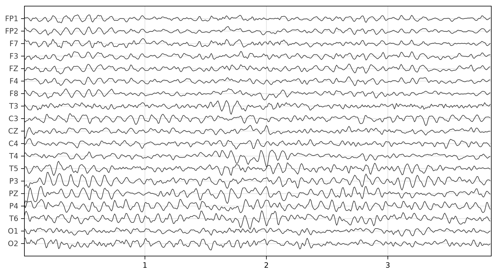

▲ Index of working examples

Plotting Multiple Datasets

The following example illustrates the inspection of PCA components. The workflow is :

• compute $u$, the principal axis of data $X$, as the eigenvector of its covariance matrix associated to the largest eigenvalue,
• compute $y$, the principal component time series (principal component score or activation), as

\[y = X u,\]

• compute $P$, the data $X$ projected on this component (subspace projection), as

\[P = y u^T,\]

• plot $X$ and overlay $P$ on the upper panel, $y$ on the lower panel.

using EEGPlot, Eegle, LinearAlgebra, CairoMakie

# read example EEG data, sampling rate and sensor labels from Eegle
X, sr = readASCII(EXAMPLE_Normative_1), 128;
sensors = readSensors(EXAMPLE_Normative_1_sensors);

u = eigvecs(covmat(X; covtype=SCM))[:, end]
y = X * reshape(u, :, 1) # using reshape, y will be a Tx1 Matrix
P = y * u'
eegplot(X, sr, sensors;
        fig_size=(814, 614),
        overlay=P,
        Y=y,
        Y_size=0.1)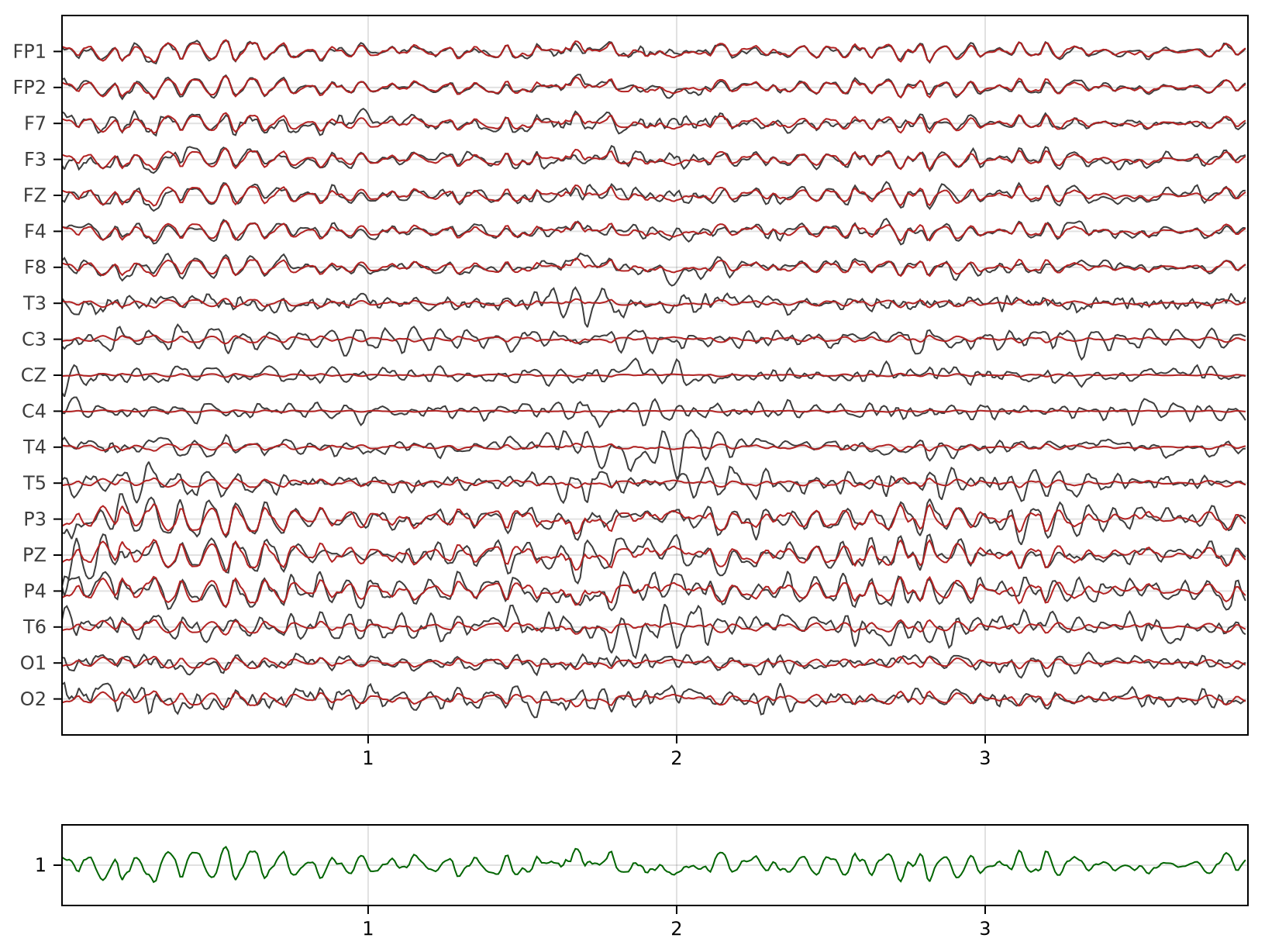

In the plot above, we see $X$ in dark grey, $P$ in brick red and $y$ in green.

▲ Index of working examples

Interactive Plots

It is obtained using the GLMakie backend instead. The syntax of eegPlot does not change at all. For example, to obtain an interactive plot of the PCA above, we would replace the first line above with:

using GLMakie

# since you may have been using CairoMakie, make sure to switch backend
GLMakie.activate!()

# Anything else is the same as above

Such plots allows interactions and look like this:

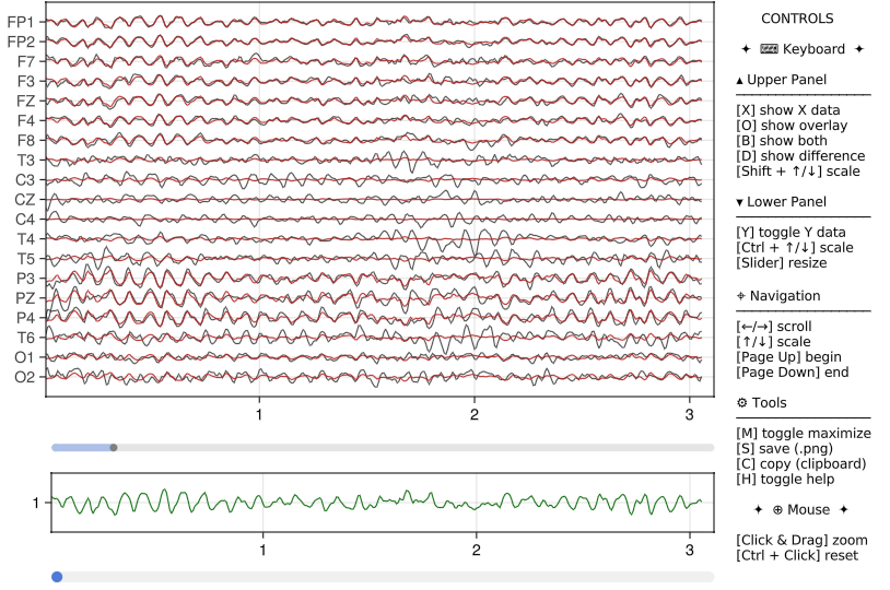
Note that in addition to static plots, interactive plots feature:

• a central slider to resize the upper and lower panels,
• a slider at the bottom of the window to scroll the data,
• an help panel summarizing the interaction controls (visible by default).
• if tags (event markers) are plotted, a legend for the tags.

▲ Index of working examples

Show Event Markers

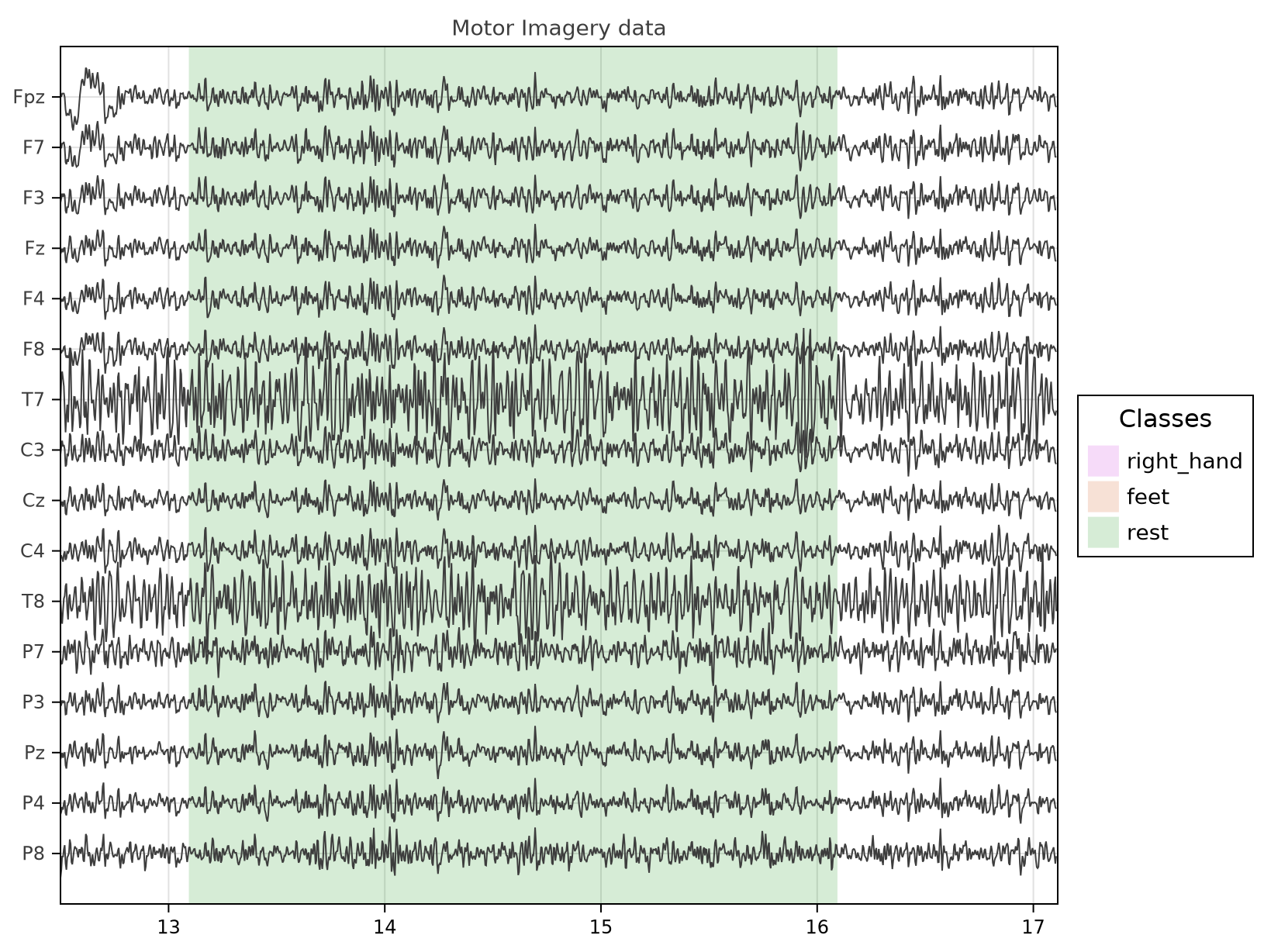
For an example of plotting EEG data with event markers, we will consider the example Motor Imagery file provided by Eegle.jl. In the recording, there are 3s trials of "rest" as well as "right hand" and "feet" movement imagination.

Tags are plotted if the stim keyword argument is provided. This argument is a Vector{Int} forming a stimulaton vector.

In this session the sampling rate is 256 samples per second and the duration of each trial is three seconds = 768 samples. Theses values are accessible in the .sr and .wl (window length) fields of the o object that will be created by Eegle's readNY function.

using EEGPlot, Eegle, CairoMakie

o = Eegle.readNY(EXAMPLE_MI_1)

eegplot(o.X, o.sr, o.sensors;
        fig_size=(814, 614),
        stim=o.stim,
        stim_labels=o.clabels, # o.clabels = ["right_hand", "feet", "rest"]
        stim_wl=o.wl,
        stim_legend_font=14,
        X_title="Motor Imagery data",
        start_pos=round(Int(o.sr*12.5)),
        px_per_sec=150
)

▲ Index of working examples

ERPs

For an example of plotting evoked potentials, we will consider the example P300 file provided by Eegle.jl. In P300 experiments, we are interested in two classes of ERP, named "target" and "nontarget". Please see Eegle.ERPs for details on the ERP computations.

using EEGPlot, Eegle, CairoMakie
CairoMakie.activate!() # let's make it static

# read the example file for the P300 BCI paradigm
o = readNY(EXAMPLE_P300_1;
            rate=4,
            upperLimit=1.2,
            bandPass=(0.5, 32)) # See Eegle.readNY

# compute means (adaptive weights and multivariate regression)
M = mean(o;
        overlapping=true,
        weights=:a) # See Eegle.mean

# target and non-target average ERP
T_ERP = M[findfirst(isequal("target"), o.clabels)]
NT_ERP = M[findfirst(isequal("nontarget"), o.clabels)]

eegplot(T_ERP, o.sr, o.sensors;
        fig_size = (300, 250),
        overlay = NT_ERP,
        Y_labels = o.sensors,
        win_length = o.wl, # trial length in samples
        px_per_sec = 160,
        init_scale = 0.8,
        X_title = "target (grey) vs. nontarget (red)",
        X_title_font_size = 10,
        X_labels_font_size = 9,
        s_labels_font_size = 8)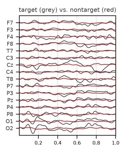

For plotting ERPs, see also UnfoldMakie.

▲ Index of working examples

🔌 API

The package exports one function only:

function eegplot(X, sr, X_labels; kwargs...)

Arguments

1. a Matrix $X \in \mathbb{R}^{T \times N_X}$ for the upper panel, where $T$ and $N_X$ are the number of samples and channels,
2. the sampling rate of dataset $X$ (Int),
3. the labels of $X$ (Vector{String}), which can be omitted.

Optional Keyword Arguments (kwargs)

💡 Examples

The examples here below assume the existence of data $X\in \mathbb{R}^{T \times N_X}$, sampling rate sr and labels sensors:

using EEGPlot, CairoMakie # or GLMakie for interactive plots

# Plot with default settings
eegplot(X, sr, sensors)

# Save a figure with large size and high quality (ppi)
# (for saving figures CairoMakie is preferable)
fig = eegplot(X, sr, sensors; 
            fig_size = (3000, 1000), 
            image_quality = 4)
save("figure.png", fig)

# Plot without providing labels for X
eegplot(X, sr)

# Two panels; Y must have the same # of samples as X
eegplot(X, sr, sensors; 
        Y = X)

# Overlay; must have the same # of samples and of channels as X
eegplot(X, sr, sensors; 
        overlay = X)

# Both overlay and two panels
eegplot(X, sr, sensors; 
        overlay = X, 
        Y = X)

# Change pixels per second (time-constant)
eegplot(X, sr, sensors; 
        px_per_sec = 280)

# Notice that the data is plotted with the same time-constant
# regardless the sampling rate. For example, doubling the sr
using Eegle # for `resample`
eegplot(resample(X, sr, 2), 256, sensors; 
        px_per_sec = 280)

# Change titles and colors
eegplot(X, sr, sensors; 
        Y = X, 
        X_title = "This the title for the upper panel",
        X_color = :blue,
        Y_title = "This the title for the lower panel",
        Y_color = :darkviolet,
        )

# Start plotting from second 2    
eegplot(X, sr, sensors; 
        start_pos = sr*2)

# Start plotting from an arbitrary sample (345)
eegplot(X, sr, sensors; 
        start_pos = 345)

# Plot from sample 345 to sample 345+sr*2 (2s)
eegplot(X, sr, sensors; 
        start_pos = 129, 
        win_length = sr*4)

🎮 Interactions

The following commands are available only in interactive mode.

⌨ Keyboard controls

▴ Upper Panel

• 'X': show the $X$ dataset
• 'O': show the $overlay$ dataset (if overlay kwarg is passed)
• 'B': show both $X$ and $overlay$ dataset (idem)
• 'D': show the difference $(X - overlay)$ (idem)
• Shift + ↑/↓: scale $X$ up/down (use scale_change kwarg)

▾ Lower Panel (if kwarg Y is passed)

• 'Y': toggle Y data (lower panel) visibility
• Ctrl + ↑/↓: scale $Y$ up/down (use scale_change kwarg)
• Slider: resize the lower panel

⌖ Navigation (apply to all visible panels)

• ←/→: scroll backward and forward the dataset(s)
• ↑/↓: scale up and down the dataset(s) (use scale_change kwarg)
• Page Up: move to begin of dataset(s)
• Page Down: move to end of dataset(s)
• T: toggle event markers visibility.

⚙ Tools

• 'M': toggle the status of the plot window (maximized/normal)
• 'Esc': restore the normal status if the window is maximized
• 'S': save the plot in the current directory as a .png file (use image_quality kwarg)
• 'C': copy the plot to the clipboard
• 'H': toggle the visibility of the help or event markers legend panels

⊕ Mouse Controls

• Click & Drag: zoom along the time-axis
• Ctrl + Click: reset the view as it was before zooming.

✍️ About the authors

Marco Congedo, Tomas Ros and Generative AI.

🌱 Contribute

Please contact the authors if you are interested in contributing.

🧭 Index

• EEGPlot.jl
• • ⚙️ Features
  • • Static and Interactive mode
    • Datasets
    • Event Markers
    • Time Constant
  • 🧩 Requirements
  • 📦 Installation
  • —͟͟͞͞★ Quick Start
  • • Static Plots
    • Plotting Multiple Datasets
    • Interactive Plots
    • Show Event Markers
    • ERPs
  • 🔌 API
  • • Arguments
    • Optional Keyword Arguments (kwargs)
  • 💡 Examples
  • 🎮 Interactions
  • • ⌨ Keyboard controls
    • ⊕ Mouse Controls
  • ✍️ About the authors
  • 🌱 Contribute
  • 🧭 Index