CCA

(1)
function cca(Cx :: SorH, Cy :: SorH, Cxy :: Mat;
             eVarCx   :: TeVaro=○,
             eVarCy   :: TeVaro=○,
             eVar     :: TeVaro=○,
             eVarMeth :: Function=searchsortedfirst,
             simple   :: Bool=false)

(2)
function cca(X::Mat, Y::Mat;
             covEst   :: StatsBase.CovarianceEstimator=SCM,
             dims     :: Into = ○,
             meanX    :: Tmean = 0,
             meanY    :: Tmean = 0,
             wX       :: Tw = ○,
             wY       :: Tw = ○,
             wXY      :: Tw = ○,
          eVarCx   :: TeVaro = ○,
          eVarCy   :: TeVaro = ○,
          eVar     :: TeVaro = ○,
          eVarMeth :: Function = searchsortedfirst,
          simple   :: Bool = false)

(3)
function cca(𝐗::VecMat, 𝐘::VecMat;
             covEst   :: StatsBase.CovarianceEstimator=SCM,
             dims     :: Into = ○,
             meanX    :: Into = 0,
             meanY    :: Into = 0,
          eVarCx   :: TeVaro = ○,
          eVarCy   :: TeVaro = ○,
          eVar     :: TeVaro = ○,
          eVarMeth :: Function = searchsortedfirst,
          simple   :: Bool = false,
       metric   :: Metric = Euclidean,
       wCx      :: Vector = [],
       wCy      :: Vector = [],
       ✓w       :: Bool = true,
       initCx   :: SorHo = nothing,
       initCy   :: SorHo = nothing,
       tol      :: Real = 0.,
       verbose  :: Bool = false)

Return a LinearFilter object:

(1) Canonical correlation analysis with, as input, real or complex:

• covariance matrix Cx of dimension $n_x⋅n_x$,
• covariance matrix Cy of dimension $n_y⋅n_y$ and
• cross-covariance matrix Cxy of dimension $n_x⋅n_y$.

Cx and Cy must be flagged as Symmetric, if real or Hermitian, if real or complex, see data input. Instead Cxy is a generic Matrix object since it is not symmetric/Hermitian, left alone square.

eVarCx, eVarCy, eVar and eVarMeth are keyword optional arguments for defining the subspace dimension $p$. Particularly:

• eVarCx and eVarCy are used to determine a subspace dimension in the whitening of Cx and Cy, i.e., in the first step of the two-step procedure descrived above in the solution section.
• eVar is used to determine the final subspace dimension using the .arev vector given by Eq. [cca.5] here above.
• eVarMeth applies to eVarCx, eVarCy and eVar.

The default values are:

• eVarCx=0.999
• eVarCy=0.999
• eVar=0.999
• eVarMeth=searchsortedfirst

If simple is set to true, $p$ is set equal to $min(n_x, n_y)$ and only the fields .F and .iF are written in the constructed object. This option is provided for low-level work when you don't need to define a subspace dimension or you want to define it by your own methods.

(2) Canonical correlation analysis with real or complex data matrices X and Y as input.

covEst, dims, meanX, meanY, wX, wY and wXY are optional keyword arguments to regulate the estimation of the covariance matrices of X and Y and their cross-covariance matrix $C_{xy}$. Particularly (See covariance matrix estimations),

• meanX is the mean argument for data matrix X.
• meanY is the mean argument for data matrix Y.
• wX is the w argument for estimating a weighted covariance matrix $C_x$.
• wY is the w argument for estimating a weighted covariance matrix $C_y$.
• wXY is the w argument for estimating a weighted cross-covariance matrix $C_{XY}$.
• covEst applies only to the estimation of $C_x$ and $C_y$.

Once $C_x$, $C_y$ and $C_{xy}$ estimated, method (1) is invoked with optional keyword arguments eVar, eVarCx, eVarCy, eVarMeth and simple. See method (1) for details.

(3) Canonical correlation analysis with two vectors of real or complex data matrices 𝐗 and 𝐘 as input. 𝐗 and 𝐘 must hold the same number of matrices and corresponding pairs of matrices therein must comprise the same number of samples.

covEst, dims, meanX and meanY are optional keyword arguments to regulate the estimation of the covariance matrices of all matrices in 𝐗 and 𝐘 and the cross-covariance matrices for all pairs of their corresponding data matrices. See method (2) and covariance matrix estimations.

A mean of these covariance matrices is computed. For the cross-covariance matrices the arithmetic mean is used. For the covariance matrices of 𝐗 and 𝐘, optional keywords arguments metric, wCx, wCy, ✓w, initCx, initCy, tol and verbose are used to allow non-Euclidean mean estimations. Particularly (see mean covariance matrix estimations),

• wCx are the weights for the covariance matrices of 𝐗,
• wCy are the weights for the covariance matrices of 𝐘,
• initCx is the initialization for the mean of the covariance matrices of 𝐗,
• initCy is the initialization for the mean of the covariance matrices of 𝐘.

By default, the arithmetic mean is computed.

Once the mean covariance and cross-covariance matrices are estimated, method (1) is invoked with optional keyword arguments eVarCx, eVarCy, eVar, eVarMeth and simple. See method (1) for details.

See also: Whitening, MCA, gCCA, mAJD.

Examples:

using Diagonalizations, LinearAlgebra, PosDefManifold, Test

# Method (1) real
n, t=10, 100
X=genDataMatrix(n, t)
Y=genDataMatrix(n, t)
Cx=Symmetric((X*X')/t)
Cy=Symmetric((Y*Y')/t)
Cxy=(X*Y')/t
cC=cca(Cx, Cy, Cxy, simple=true)
@test cC.F[1]'*Cx*cC.F[1]≈I
@test cC.F[2]'*Cy*cC.F[2]≈I
D=cC.F[1]'*Cxy*cC.F[2]
@test norm(D-Diagonal(D))+1. ≈ 1.

# Method (1) complex
Xc=genDataMatrix(ComplexF64, n, t)
Yc=genDataMatrix(ComplexF64, n, t)
Cxc=Hermitian((Xc*Xc')/t)
Cyc=Hermitian((Yc*Yc')/t)
Cxyc=(Xc*Yc')/t
cCc=cca(Cxc, Cyc, Cxyc, simple=true)
@test cCc.F[1]'*Cxc*cCc.F[1]≈I
@test cCc.F[2]'*Cyc*cCc.F[2]≈I
Dc=cCc.F[1]'*Cxyc*cCc.F[2]
@test norm(Dc-Diagonal(Dc))+1. ≈ 1.


# Method (2) real
cXY=cca(X, Y, simple=true)
@test cXY.F[1]'*Cx*cXY.F[1]≈I
@test cXY.F[2]'*Cy*cXY.F[2]≈I
D=cXY.F[1]'*Cxy*cXY.F[2]
@test norm(D-Diagonal(D))+1. ≈ 1.
@test cXY==cC

# Method (2) complex
cXYc=cca(Xc, Yc, simple=true)
@test cXYc.F[1]'*Cxc*cXYc.F[1]≈I
@test cXYc.F[2]'*Cyc*cXYc.F[2]≈I
Dc=cXYc.F[1]'*Cxyc*cXYc.F[2]
@test norm(Dc-Diagonal(Dc))+1. ≈ 1.
@test cXYc==cCc


# Method (3) real
# canonical correlation analysis of the average covariance and cross-covariance
k=10
Xset=[genDataMatrix(n, t) for i=1:k]
Yset=[genDataMatrix(n, t) for i=1:k]

c=cca(Xset, Yset)

# ... selecting subspace dimension allowing an explained variance = 0.9
c=cca(Xset, Yset; eVar=0.9)

# ... subtracting the mean from the matrices in Xset and Yset
c=cca(Xset, Yset; meanX=nothing, meanY=nothing, eVar=0.9)

# cca on the average of the covariance and cross-covariance matrices
# computed along dims 1
c=cca(Xset, Yset; dims=1, eVar=0.9)

# name of the filter
c.name

using Plots
# plot regularized accumulated eigenvalues
plot(c.arev)

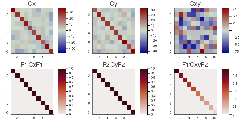
# plot the original covariance and cross-covariance matrices
# and their transformed counterpart
 CxyMax=maximum(abs.(Cxy));
 h1 = heatmap(Cxy, clim=(-CxyMax, CxyMax), title="Cxy", yflip=true, c=:bluesreds);
 D=cC.F[1]'*Cxy*cC.F[2];
 Dmax=maximum(abs.(D));
 h2 = heatmap(D, clim=(0, Dmax), title="F1'CxyF2", yflip=true, c=:amp);
 CxMax=maximum(abs.(Cx));
 h3 = heatmap(Cx, clim=(-CxMax, CxMax), title="Cx", yflip=true, c=:bluesreds);
 h4 = heatmap(cC.F[1]'*Cx*cC.F[1], clim=(0, 1), title="F1'CxF1", yflip=true, c=:amp);
 CyMax=maximum(abs.(Cy));
 h5 = heatmap(Cy, clim=(-CyMax, CyMax), title="Cy", yflip=true, c=:bluesreds);
 h6 = heatmap(cC.F[2]'*Cy*cC.F[2], clim=(0, 1), title="F2'CyF2", yflip=true, c=:amp);
 📈=plot(h3, h5, h1, h4, h6, h2, size=(800,400))
# savefig(📈, homedir()*"\Documents\Code\julia\Diagonalizations\docs\src\assets\FigCCA.png")

# Method (3) complex
# canonical correlation analysis of the average covariance and cross-covariance
k=10
Xcset=[genDataMatrix(ComplexF64, n, t) for i=1:k]
Ycset=[genDataMatrix(ComplexF64, n, t) for i=1:k]

cc=cca(Xcset, Ycset)

# ... selecting subspace dimension allowing an explained variance = 0.9
cc=cca(Xcset, Ycset; eVar=0.9)

# ... subtracting the mean from the matrices in Xset and Yset
cc=cca(Xcset, Ycset; meanX=nothing, meanY=nothing, eVar=0.9)

# cca on the average of the covariance and cross-covariance matrices
# computed along dims 1
cc=cca(Xcset, Ycset; dims=1, eVar=0.9)

# name of the filter
cc.name